Illustration of the Back-and-Forth Method on WOP with a 1-D example#
import sys
import os
sys.path.append(os.path.abspath("../.."))

import numpy as np
import numpy.ma as ma
from scipy.fftpack import dctn, idctn
import matplotlib.pyplot as plt
from time import time
from BFOT.BFOT import BFM
import cProfile
import pstats
import math
---------------------------------------------------------------------------
ModuleNotFoundError                       Traceback (most recent call last)
Cell In[1], line 10
      8 import matplotlib.pyplot as plt
      9 from time import time
---> 10 from BFOT.BFOT import BFM
     11 import cProfile
     12 import pstats

File ~/work/BFOT/BFOT/BFOT/BFOT.py:2
      1 import numpy as np
----> 2 import numba
      3 from numba import prange
      4 from scipy.signal import convolve2d

ModuleNotFoundError: No module named 'numba'
plt.rcParams['figure.figsize'] = (13, 8)
plt.rcParams['image.cmap'] = 'viridis'

# Function definitions
def initialize_kernel(n1, n2):
    xx, yy = np.meshgrid(np.linspace(0, np.pi, n1, False), np.linspace(0, np.pi, n2, False))
    kernel = 2 * n1 * n1 * (1 - np.cos(xx)) + 2 * n2 * n2 * (1 - np.cos(yy))
    kernel[0, 0] = 1  # to avoid dividing by zero
    return kernel

def dct2(a):
    #discrete cosine transform
    return dctn(a, norm='ortho')

def idct2(a):
    #inverse discrete cosine transform
    return idctn(a, norm='ortho')

def update_potential(phi, rho, nu, kernel, sigma):
    n1, n2 = nu.shape
    rho -= nu
    workspace = dct2(rho) / kernel
    workspace[0, 0] = 0
    workspace = idct2(workspace)
    phi += sigma * workspace
    h1 = np.sum(workspace * rho) / (n1 * n2)
    return h1

def compute_w2(phi, psi, mu, nu, x, y):
    n1, n2 = mu.shape
    return np.sum(0.5 * (x * x + y * y) * (mu + nu) - nu * phi.reshape((n1, n2)) - mu * psi.reshape((n1, n2))) / (n1 * n2)

def compute_w2_wop(phi, psi, mu, nu, x, y, m_mu, m_nu):
    n1, n2 = mu.shape
    return np.sum(0.5 * (x * x + y * y) * (mu + nu) - nu * phi.reshape((n1, n2)) - mu * psi.reshape((n1, n2)) + (m_mu - m_nu) ** 2) / (n1 * n2)

def stepsize_update(sigma, value, oldValue, gradSq):
    scaleDown = 0.95
    scaleUp = 1 / scaleDown
    upper = 0.75
    lower = 0.25
    diff = value - oldValue
    if diff > gradSq * sigma * upper:
        return sigma * scaleUp
    elif diff < gradSq * sigma * lower:
        return sigma * scaleDown
    return sigma
# use the pudhforward function in the c file

import matplotlib.pyplot as plt
import numpy as np

def compute_ot(phi, psi, bf, sigma):
    kernel = initialize_kernel(n2, n1)
    rho = np.copy(mu)
    oldValue = compute_w2(phi, psi, mu, nu, x, y)

    for k in range(numIters + 1):
        # Perform gradient and potential updates
        gradSq = update_potential(phi, rho, nu, kernel, sigma)
        bf.ctransform(psi, phi)
        bf.ctransform(phi, psi)
        value = compute_w2(phi, psi, mu, nu, x, y)
        sigma = stepsize_update(sigma, value, oldValue, gradSq)
        oldValue = value
        bf.pushforward(rho, phi, nu)
        # Update potential and push forward for psi
        gradSq = update_potential(psi, rho, mu, kernel, sigma)
        bf.ctransform(phi, psi)
        bf.ctransform(psi, phi)
        bf.pushforward(rho, psi, mu)

        # Logging the values
        if k % 10 == 0:
            print(f'iter {k:4d},   W2 value: {value:.6e},   H1 err: {gradSq:.2e}')
        #if k % 10 == 0:
            #print(bf.xMap, bf.yMap)

        # Update stepsize and oldValue for next iteration
        sigma = stepsize_update(sigma, value, oldValue, gradSq)
        oldValue = value

def compute_ot_wop(phi, psi, bf, sigma):
    kernel = initialize_kernel(n2, n1)
    rho = np.copy(mu)
    oldValue = compute_w2_wop(phi, psi, mu, nu, x, y, m_mu, m_nu)

    for k in range(numIters + 1):
        # Perform gradient and potential updates
        gradSq = update_potential(phi, rho, nu, kernel, sigma)
        bf.ctransform(psi, phi)
        bf.ctransform(phi, psi)
        value = compute_w2_wop(phi, psi, mu, nu, x, y, m_mu, m_nu)
        sigma = stepsize_update(sigma, value, oldValue, gradSq)
        oldValue = value
        bf.pushforward(rho, phi, nu)
        # Update potential and push forward for psi
        gradSq = update_potential(psi, rho, mu, kernel, sigma)
        bf.ctransform(phi, psi)
        bf.ctransform(psi, phi)
        bf.pushforward(rho, psi, mu)

        # Logging the values
        if k % 10 == 0:
            print(f'iter {k:4d},   W2 value: {value:.6e},   H1 err: {gradSq:.2e}')
        #if k % 10 == 0:
            #print(bf.xMap, bf.yMap)

        # Update stepsize and oldValue for next iteration
        sigma = stepsize_update(sigma, value, oldValue, gradSq)
        oldValue = value
# functions for calculating the pushforward by mass
import numpy as np
from scipy.signal import convolve2d

def sampling_pushforward_jit(rho, xMap, yMap, mu, n1, n2, totalMass):
    """
    Compute the pushforward measure using a sampling-based method.

    Parameters:
        rho (np.ndarray): Array of shape (n1, n2) to store the resulting density.
        xMap (np.ndarray): The computed x-coordinate mapping (shape must be (n1+1, n2+1)).
        yMap (np.ndarray): The computed y-coordinate mapping (shape must be (n1+1, n2+1)).
        mu (np.ndarray): Source measure (density) of shape (n1, n2).
        n1 (int): Number of grid points in the x-direction.
        n2 (int): Number of grid points in the y-direction.
        totalMass (float): The total mass to normalize the output density.
    """
    # 1) Clear out rho
    pcount = n1 * n2
    for i in range(n1):
        for j in range(n2):
            rho[i, j] = 0.0

    # 2) Loop over each cell and subdivide
    for i in range(n1):
        for j in range(n2):
            mass = mu[i, j]
            if mass > 0.0:
                # Compute stretches along x and y
                xStretch0 = abs(xMap[i,     j+1] - xMap[i,     j])
                xStretch1 = abs(xMap[i + 1, j+1] - xMap[i + 1, j])
                yStretch0 = abs(yMap[i + 1, j]   - yMap[i,     j])
                yStretch1 = abs(yMap[i + 1, j+1] - yMap[i,     j+1])

                xStretch = max(xStretch0, xStretch1)
                yStretch = max(yStretch0, yStretch1)

                xSamples = max(int(n1 * xStretch), 1)
                ySamples = max(int(n2 * yStretch), 1)

                factor = 1.0 / (xSamples * ySamples)

                # 3) Sample within the cell
                for l in range(ySamples):
                    b = (l + 0.5) / ySamples
                    for k in range(xSamples):
                        a = (k + 0.5) / xSamples

                        # Bilinear interpolation for xMap and yMap
                        xPoint = (
                            (1 - b)*(1 - a)*xMap[i,     j] +
                            (1 - b)*a      *xMap[i,     j+1] +
                            b      *(1 - a)*xMap[i + 1, j] +
                            a*b            *xMap[i + 1, j+1]
                        )
                        yPoint = (
                            (1 - b)*(1 - a)*yMap[i,     j] +
                            (1 - b)*a      *yMap[i,     j+1] +
                            b      *(1 - a)*yMap[i + 1, j] +
                            a*b            *yMap[i + 1, j+1]
                        )

                        # Convert continuous coordinates to discrete indices
                        X = xPoint * n1 - 0.5
                        Y = yPoint * n2 - 0.5

                        xIndex = int(X)
                        yIndex = int(Y)
                        xFrac = X - xIndex
                        yFrac = Y - yIndex
                        xOther = xIndex + 1
                        yOther = yIndex + 1

                        # Clamp indices
                        xIndex = max(0, min(xIndex, n1-1))
                        xOther = max(0, min(xOther, n1-1))
                        yIndex = max(0, min(yIndex, n2-1))
                        yOther = max(0, min(yOther, n2-1))

                        # 4) Distribute mass using bilinear weights
                        w00 = (1.0 - xFrac)*(1.0 - yFrac)
                        w01 = (1.0 - xFrac)*yFrac
                        w10 = xFrac*(1.0 - yFrac)
                        w11 = xFrac*yFrac

                        rho[yIndex, xIndex] += w00 * mass * factor
                        rho[yOther, xIndex] += w01 * mass * factor
                        rho[yIndex, xOther] += w10 * mass * factor
                        rho[yOther, xOther] += w11 * mass * factor

    # 5) Normalize so that the total measure equals totalMass
    sum_rho = 0.0
    for i in range(n1):
        for j in range(n2):
            sum_rho += rho[i, j]
    sum_rho /= pcount  # average density
    if sum_rho > 0.0:
        scale = totalMass / sum_rho
        for i in range(n1):
            for j in range(n2):
                rho[i, j] *= scale

def cal_pushforward_map(dual, n1, n2):
    """
    Compute the pushforward map (xMap and yMap) from the dual variable.

    Parameters:
        dual (np.ndarray): The dual variable (often denoted phi).
        n1 (int): Number of grid points in the x-direction.
        n2 (int): Number of grid points in the y-direction.

    Returns:
        xMap (np.ndarray), yMap (np.ndarray): The computed mapping arrays.
    """
    kernel = np.array([[0.25, 0.25],
                       [0.25, 0.25]])
    dual_padded = np.pad(dual, ((1, 1), (1, 1)), mode="edge")
    interpolate_function = convolve2d(dual_padded, kernel, mode="valid")
    interpolate_function_padded = np.pad(interpolate_function, ((1, 1), (1, 1)), mode="edge")
    xMap = 0.5 * n2 * (interpolate_function_padded[1:-1, 2:] - interpolate_function_padded[1:-1, :-2])
    yMap = 0.5 * n1 * (interpolate_function_padded[2:, 1:-1] - interpolate_function_padded[:-2, 1:-1])
    return xMap, yMap

def pushforward_mass(phi, nu, n1, n2):
    """
    Perform the pushforward of the measure 'nu' using the dual variable 'phi',
    and store the resulting measure in 'rho'.

    Parameters:
        rho (np.ndarray): An (n1 x n2) array to store the pushforward measure.
        phi (np.ndarray): The dual variable used to compute the pushforward map.
        nu (np.ndarray): The source measure (density) on the grid.
        n1 (int): Number of grid points in the x-direction.
        n2 (int): Number of grid points in the y-direction.
        totalMass (float): The total mass for normalization.

    Returns:
        np.ndarray: The updated pushforward measure stored in 'rho'.
    """
    rho = np.zeros((n1, n2))
    totalMass = np.sum(nu) / (n1 * n2)
    # Compute the pushforward maps based on phi
    xMap, yMap = cal_pushforward_map(phi, n1, n2)

    # Use the sampling pushforward method to update rho
    sampling_pushforward_jit(rho, xMap, yMap, nu, n1, n2, totalMass)

    return rho

def plot_interpolation_wop(mu, nu, phi, psi, bf, x, y, n1, n2, m_mu, m_nu, n_fig=11):
    """
    Plots the discrete geodesic interpolation between mu and nu
    using the given potentials phi and psi.

    Parameters
    ----------
    mu : 2D array (n2, n1)
        Source measure.
    nu : 2D array (n2, n1)
        Target measure.
    phi, psi : 2D arrays (n2, n1)
        Kantorovich potentials.
    bf : BFM object
        Instance of the Semi-discrete solver that has a pushforward method.
    x, y : 2D arrays (n2, n1)
        Grid coordinates.
    n_fig : int
        Number of frames to plot (including t=0 and t=1).
    """
    fig, ax = plt.subplots(1, n_fig, figsize=(20, 8))
    for axi in ax:
        axi.axis('off')

    # Use the same max for color scaling
    vmax = mu.max()

    # Allocate arrays for intermediate pushforwards
    interpolate = np.zeros_like(mu)
    rho_fwd = np.zeros_like(mu)
    rho_bwd = np.zeros_like(mu)

    # "Reference" potential = 0.5*(x² + y²)
    phi_0 = 0.5 * (x**2 + y**2)

    fig, ax = plt.subplots(1, n_fig, figsize=(24,4), sharex=True, sharey=True)

    # Generate intermediate frames
    for i in range(0, n_fig):
        t = (1 - np.cos(math.pi * i / (n_fig - 1))) / 2

        # Blend potentials in 2D form
        # psi_t interpolates from phi_0 to psi
        # phi_t interpolates from phi_0 to phi
        psi_t = (1 - t) * phi_0 + t * psi
        phi_t = t * phi_0 + (1 - t) * phi

        # Pushforward mu by psi_t
        bf.pushforward(rho_fwd, psi_t, mu)

        # Pushforward nu by phi_t
        bf.pushforward(rho_bwd, phi_t, nu)

        # reverse the oushforwards by mass
        phi_mu_re = 0.5 * ((1/m_mu) * (x * x) + (1/m_mu) * y * y)
        phi_nu_re = 0.5 * ((1/m_nu) * (x * x) + (1/m_nu) * y * y)
        rho_fwd = pushforward_mass(phi_mu_re, rho_fwd, n1, n2)
        rho_bwd = pushforward_mass(phi_nu_re, rho_bwd, n1, n2)

        # Convex combination of the two pushforwards
        interpolate = (1 - t) * rho_fwd + t * rho_bwd

        # Plot the interpolation
        ax[i].imshow(interpolate, origin='lower', extent=(0, 1, 0, 1), vmax=vmax)
        ax[i].set_title(f"$t={t:.2f}$")
1D-distributions with equal mass#
import math
# 1-D distribution
n1 = 256
n2 = 256
x = np.linspace(0, 2 * math.pi, n2) # Generate n equally spaced points between 0 and 2pi
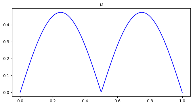
mu0 = np.abs(np.sin(x))
x = x/(2 * math.pi)
mu0 *= n2 / np.sum(mu0)
# visualize mu distribution
plt.figure(figsize=(8, 4))
plt.plot(x, mu0, color='blue')
plt.title("$\\mu$")
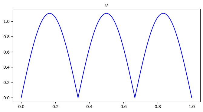
x = np.linspace(0, 3 * math.pi, n2) # Generate n equally spaced points between 0 and 2pi
nu0 = np.abs(np.cos(x + 0.5 * math.pi))
x = x/(3 * math.pi)
nu0 *= n2 / np.sum(nu0)
# visualize nu distribution
plt.figure(figsize=(8, 4))
plt.plot(x, nu0, color='blue')
plt.title("$\\nu$")
mu = np.zeros((n1, n2))
nu = np.zeros((n1, n2))
mu[n1//2, ] = mu0
nu[n1//2, ] = nu0
x, y = np.meshgrid(np.linspace(0.5 / n1, 1 - 0.5 / n1, n1), np.linspace(0.5 / n2, 1 - 0.5 / n2, n2))
phi = 0.5 * (x * x + y * y)
psi = 0.5 * (x * x + y * y)
numIters = 50
sigma = 4 / np.maximum(mu.max(), nu.max())
def main():
    bf = BFM(n1, n2, mu)
    compute_ot(phi, psi, bf, sigma)
    plot_interpolation_wop(mu, nu, phi, psi, bf, x, y, n1, n2, m_mu, m_nu, n_fig=11)

if __name__ == "__main__":
    profiler = cProfile.Profile()
    profiler.enable()

    main()

    profiler.disable()
    stats = pstats.Stats(profiler)
    stats.sort_stats('tottime').print_stats(10)
Exception ignored When destroying _lsprof profiler:
Traceback (most recent call last):
  File "/var/folders/55/y04y93j97zjfs37qlvlf3r1m0000gn/T/ipykernel_89671/537028364.py", line 8, in <module>
RuntimeError: Cannot install a profile function while another profile function is being installed
iter    0,   W2 value: 5.510644e-07,   H1 err: 1.92e-07
iter   10,   W2 value: 3.537803e-06,   H1 err: 1.38e-08
iter   20,   W2 value: 3.694454e-06,   H1 err: 4.56e-09
iter   30,   W2 value: 3.711893e-06,   H1 err: 2.90e-09
iter   40,   W2 value: 3.715814e-06,   H1 err: 2.45e-09
iter   50,   W2 value: 3.716935e-06,   H1 err: 2.33e-09
---------------------------------------------------------------------------
NameError                                 Traceback (most recent call last)
Cell In[20], line 10
      7 profiler = cProfile.Profile()
      8 profiler.enable()
---> 10 main()
     12 profiler.disable()
     13 stats = pstats.Stats(profiler)

Cell In[20], line 4, in main()
      2 bf = BFM(n1, n2, mu)
      3 compute_ot(phi, psi, bf, sigma)
----> 4 plot_interpolation_wop(mu, nu, phi, psi, bf, x, y, n1, n2, m_mu, m_nu, n_fig=11)

NameError: name 'm_mu' is not defined
WOP(1-D distributions with different mass)#
# set up mu and nu with different total mass
import math
# 1-D distribution
n1 = 256
n2 = 256

x = np.linspace(0, 2 * math.pi, n2)  # Generate n equally spaced points between 0 and 2pi
mu0 = np.abs(np.sin(x))
x = x/(2 * math.pi)
mu0 *= n2 / np.sum(mu0)
mu0 *= 0.3
# visualize mu distribution
plt.figure(figsize=(8, 4))
plt.plot(x, mu0, color='blue')
plt.title("$\\mu$")

x = np.linspace(0, 3 * math.pi, n2)  # Generate n equally spaced points between 0 and 2pi
nu0 = np.abs(np.cos(x + 0.5 * math.pi))
x = x/(3 * math.pi)
nu0 *= n2 / np.sum(nu0)
nu0 *= 0.7
# visualize nu distribution
plt.figure(figsize=(8, 4))
plt.plot(x, nu0, color='blue')
plt.title("$\\nu$")

mu = np.zeros((n1, n2))
nu = np.zeros((n1, n2))

mu[n1//2, ] = mu0
nu[n1//2, ] = nu0
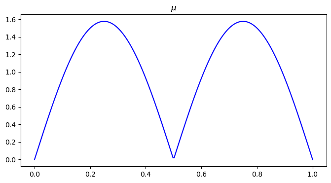
1-D example with unequal mass#
# set up mu and nu with different total mass
import math
# 1-D distribution
n1 = 256
n2 = 256
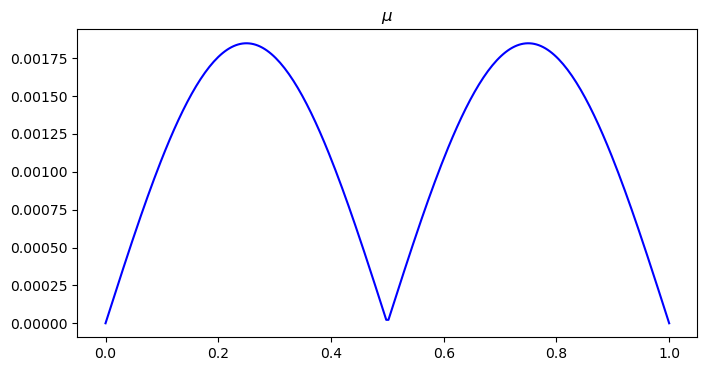
x = np.linspace(0, 2 * math.pi, n2) # Generate n equally spaced points between 0 and 2pi
mu0 = np.abs(np.sin(x))
x = x/(2 * math.pi)
mu0 *= n2 / np.sum(mu0)
mu0 *= 0.3 / n2
# visualize mu distribution
plt.figure(figsize=(8, 4))
plt.plot(x, mu0, color='blue')
plt.title("$\\mu$")
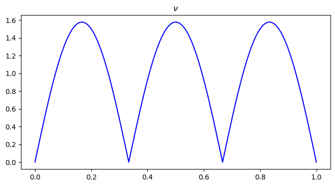
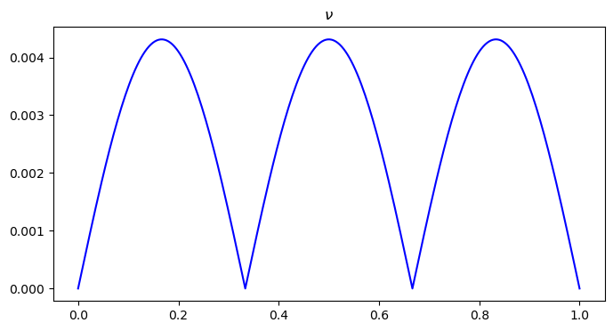
x = np.linspace(0, 3 * math.pi, n2) # Generate n equally spaced points between 0 and 2pi
nu0 = np.abs(np.cos(x + 0.5 * math.pi))
x = x/(3 * math.pi)
nu0 *= n2 / np.sum(nu0)
nu0 *= 0.7 / n2
# visualize nu distribution
plt.figure(figsize=(8, 4))
plt.plot(x, nu0, color='blue')
plt.title("$\\nu$")
mu = np.zeros((n1, n2))
nu = np.zeros((n1, n2))
mu[n1//2, ] = mu0
nu[n1//2, ] = nu0
# get the mass of the two distributions
m_mu = np.sum(mu)
m_nu = np.sum(nu)
x, y = np.meshgrid(np.linspace(0.5 / n1, 1 - 0.5 / n1, n1), np.linspace(0.5 / n2, 1 - 0.5 / n2, n2))
phi = 0.5 * (x * x + y * y)
psi = 0.5 * (x * x + y * y)
phi_mu = 0.5 * (m_mu * (x * x) + y * y)
phi_nu = 0.5 * (m_nu * (x * x) + y * y)
numIters = 30
sigma = 4 / np.maximum(mu.max(), nu.max())
# normalize the two distributions
mu *= (n1*n2) / np.sum(mu)
nu *= (n1*n2) / np.sum(nu)
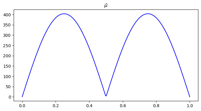
# visualize the normalized mu distribution
x = np.linspace(0, 1, n1)
plt.figure(figsize=(8, 4))
plt.plot(x, mu[n1//2, ], color='blue')
plt.title("$\\bar{\\mu}$")
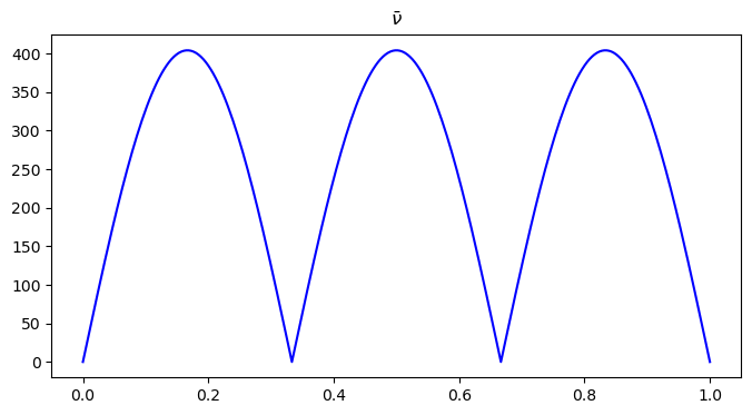
# visualize the normalized nu distribution
x = np.linspace(0, 1, n2)
plt.figure(figsize=(8, 4))
plt.plot(x, nu[n1//2, ], color='blue')
plt.title("$\\bar{\\nu}$")
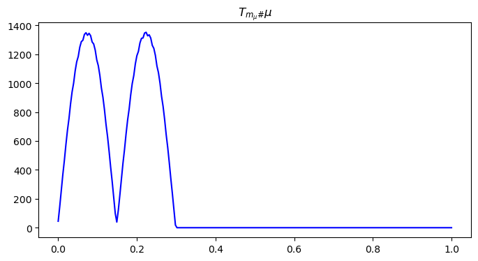
# Call pushforward to compute the pushforward measure
mu = pushforward_mass(phi_mu, mu, n1, n2)
# visualize the pushed mu distribution
x = np.linspace(0, 1, n1)
plt.figure(figsize=(8, 4))
plt.plot(x, mu[n1//2, ], color='blue')
plt.title("$T_{m_{\\mu}\#}\\mu$")
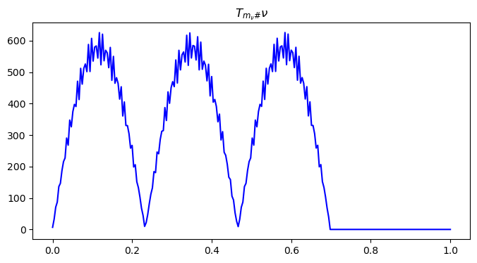
nu = pushforward_mass(phi_nu, nu, n1, n2)
# visualize the pushed nu distribution
x = np.linspace(0, 1, n2)
plt.figure(figsize=(8, 4))
plt.plot(x, nu[n1//2, ], color='blue')
plt.title("$T_{m_{\\nu}\#}\\nu$")
def main():
bf = BFM(n1, n2, mu)
compute_ot_wop(phi, psi, bf, sigma)
plot_interpolation_wop(mu, nu, phi, psi, bf, x, y, n1, n2, m_mu, m_nu)
if __name__ == "__main__":
profiler = cProfile.Profile()
profiler.enable()
main()
profiler.disable()
stats = pstats.Stats(profiler)
stats.sort_stats('tottime').print_stats(10)
Exception ignored When destroying _lsprof profiler:
Traceback (most recent call last):
  File "/var/folders/55/y04y93j97zjfs37qlvlf3r1m0000gn/T/ipykernel_89671/1273600590.py", line 81, in <module>
RuntimeError: Cannot install a profile function while another profile function is being installed
---------------------------------------------------------------------------
QhullError                                Traceback (most recent call last)
Cell In[26], line 83
     80 profiler = cProfile.Profile()
     81 profiler.enable()
---> 83 main()
     85 profiler.disable()
     86 stats = pstats.Stats(profiler)

Cell In[26], line 76, in main()
     74 def main():
     75     bf = BFM(n1, n2, mu)
---> 76     compute_ot_wop(phi, psi, bf, sigma)
     77     plot_interpolation_wop(mu, nu, phi, psi, bf, x, y, n1, n2, m_mu, m_nu)

Cell In[4], line 92, in compute_ot_wop(phi, psi, bf, sigma)
     90 gradSq = update_potential(phi, rho, nu, kernel, sigma)
     91 bf.ctransform(psi, phi)
---> 92 bf.ctransform(phi, psi)
     93 value = compute_w2_wop(phi, psi, mu, nu, x, y, m_mu, m_nu)
     94 sigma = stepsize_update(sigma, value, oldValue, gradSq)

File ~/Documents/BFOT/BFOT/BFOT.py:135, in BFM.ctransform(self, dual, phi)
    134 def ctransform(self, dual, phi):
--> 135     self.compute_2d_dual_inside(dual, phi)

File ~/Documents/BFOT/BFOT/BFOT.py:155, in BFM.compute_2d_dual_inside(self, dual, u)
    152 temp = np.empty((self.n1, self.n2))
    154 for i in range(self.n1):
--> 155     self.compute_dual(temp[i, :], u[i, :])
    157 temp = - temp
    158 for j in range(self.n2):

File ~/Documents/BFOT/BFOT/BFOT.py:168, in BFM.compute_dual(self, dual, u)
    165 points = np.column_stack((x_coords, u))
    167 # Compute convex hull
--> 168 hull = ConvexHull(points)
    170 # Extract hull vertices
    171 hull_indices = hull.vertices

File _qhull.pyx:2431, in scipy.spatial._qhull.ConvexHull.__init__()

File _qhull.pyx:353, in scipy.spatial._qhull._Qhull.__init__()

QhullError: QH6154 Qhull precision error: Initial simplex is flat (facet 1 is coplanar with the interior point)

While executing:  | qhull i Qt
Options selected for Qhull 2019.1.r 2019/06/21:
  run-id 504515528  incidence  Qtriangulate  _pre-merge  _zero-centrum
  _max-width  1  Error-roundoff 1e-13  _one-merge 5e-13  _near-inside 2.5e-12
  Visible-distance 2e-13  U-max-coplanar 2e-13  Width-outside 4e-13
  _wide-facet 1.2e-12  _maxoutside 6e-13

The input to qhull appears to be less than 2 dimensional, or a
computation has overflowed.

Qhull could not construct a clearly convex simplex from points:
- p1(v3): 0.0039 1.5e+02
- p255(v2):     1 1.5e+02
- p0(v1):     0 1.5e+02

The center point is coplanar with a facet, or a vertex is coplanar
with a neighboring facet.  The maximum round off error for
computing distances is 1e-13.  The center point, facets and distances
to the center point are as follows:

center point   0.3333    149.2

facet p255 p0 distance= -2.8e-14
facet p1 p0 distance= 2.8e-14
facet p1 p255 distance=    0

These points either have a maximum or minimum x-coordinate, or
they maximize the determinant for k coordinates.  Trial points
are first selected from points that maximize a coordinate.

The min and max coordinates for each dimension are:
  0:         0    0.9961  difference= 0.9961
  1:       149     149.6  difference= 0.5895

If the input should be full dimensional, you have several options that
may determine an initial simplex:
  - use 'QJ'  to joggle the input and make it full dimensional
  - use 'QbB' to scale the points to the unit cube
  - use 'QR0' to randomly rotate the input for different maximum points
  - use 'Qs'  to search all points for the initial simplex
  - use 'En'  to specify a maximum roundoff error less than 1e-13.
  - trace execution with 'T3' to see the determinant for each point.

If the input is lower dimensional:
  - use 'QJ' to joggle the input and make it full dimensional
  - use 'Qbk:0Bk:0' to delete coordinate k from the input.  You should
    pick the coordinate with the least range.  The hull will have the
    correct topology.
  - determine the flat containing the points, rotate the points
    into a coordinate plane, and delete the other coordinates.
  - add one or more points to make the input full dimensional.
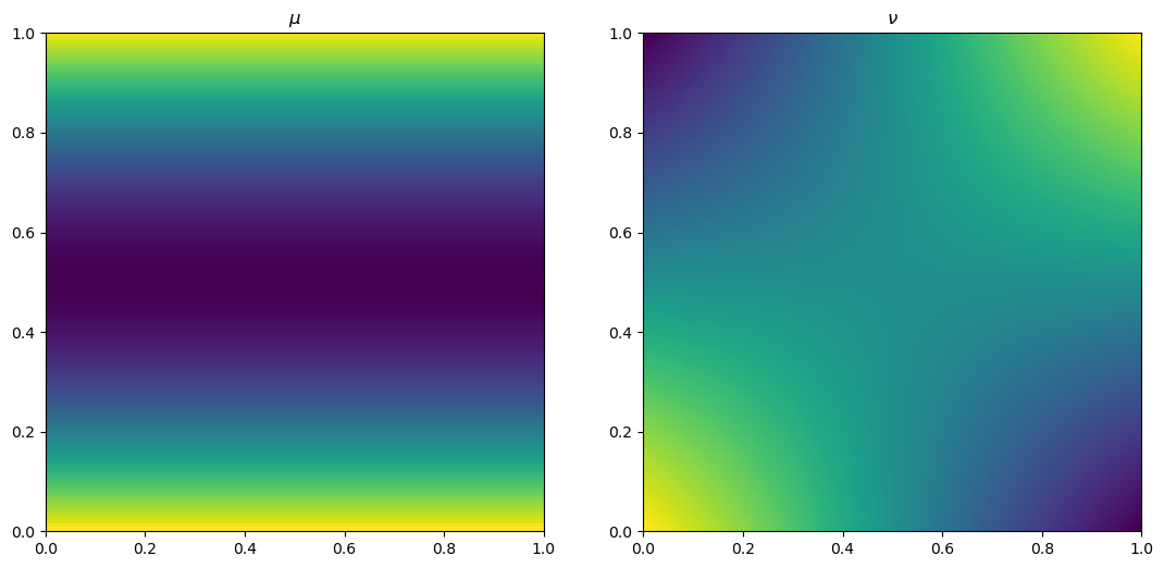
2-D example of unequal mass#
n1 = 128
n2 = 128
mu = np.zeros((n1,n2))
nu = np.zeros((n1,n2))

for i in range(n1):
    for j in range(n2):
        mu[i,j] = np.cos(np.pi*(128/n1)*(i/n1+0.5)) + 1
        nu[i,j] = np.cos(np.pi*(64/n1)*(i/n1+0.5))*np.cos(np.pi*(64/n1)*(j/n2+0.5)) + 1

fig, ax = plt.subplots(1, 2)
ax[0].imshow(mu, origin='lower', extent=(0, 1, 0, 1))
ax[0].set_title("$\\mu$")
ax[1].imshow(nu, origin='lower', extent=(0, 1, 0, 1))
ax[1].set_title("$\\nu$")

m_mu = np.sum(mu)
m_nu = np.sum(nu)
print(f'total mass of mu = {m_mu}, total mass of nu = {m_nu}')
total mass of mu = 5954.14525356209, total mass of nu = 16384.5
mu = mu/m_nu
nu = nu/m_nu
fig, ax = plt.subplots(1, 2)
ax[0].imshow(mu, origin='lower', extent=(0, 1, 0, 1))
ax[0].set_title("$\\mu$")
ax[1].imshow(nu, origin='lower', extent=(0, 1, 0, 1))
ax[1].set_title("$\\nu$")
m_mu = np.sum(mu)
m_nu = np.sum(nu)
print(f'total mass of mu = {m_mu}, total mass of nu = {m_nu}')
total mass of mu = 0.36340109576502727, total mass of nu = 1.0
x, y = np.meshgrid(np.linspace(0.5 / n1, 1 - 0.5 / n1, n1), np.linspace(0.5 / n2, 1 - 0.5 / n2, n2))
phi = 0.5 * (x * x + y * y)
psi = 0.5 * (x * x + y * y)
phi_mu = 0.5 * (m_mu * (x * x) + m_mu * (y * y))
phi_nu = 0.5 * (x * x + y * y)
numIters = 30
sigma = 4 / np.maximum(mu.max(), nu.max())
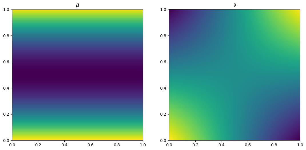
# normalize the two distributions
mu *= (n1*n2) / np.sum(mu)
nu *= (n1*n2) / np.sum(nu)
# visualize the normalized mu distribution
fig, ax = plt.subplots(1, 2)
ax[0].imshow(mu, origin='lower', extent=(0, 1, 0, 1))
ax[0].set_title("$\\bar{\\mu}$")
ax[1].imshow(nu, origin='lower', extent=(0, 1, 0, 1))
ax[1].set_title("$\\bar{\\nu}$")
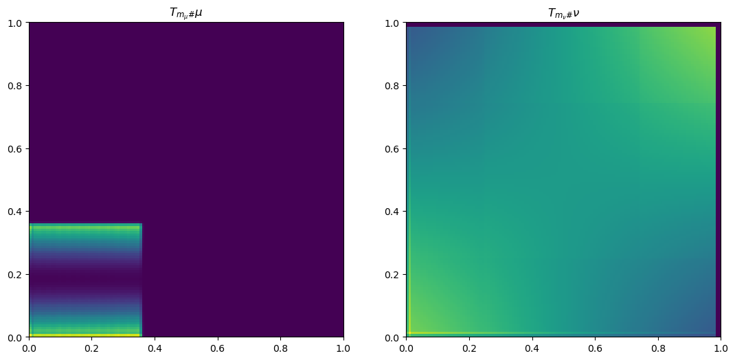
# Call pushforward to compute the pushforward measure
mu = pushforward_mass(phi_mu, mu, n1, n2)
nu = pushforward_mass(phi_nu, nu, n1, n2)
# visualize the pushed nu distribution
fig, ax = plt.subplots(1, 2)
ax[0].imshow(mu, origin='lower', extent=(0, 1, 0, 1))
ax[0].set_title("$T_{m_{\\mu}\#}\\mu$")
ax[1].imshow(nu, origin='lower', extent=(0, 1, 0, 1))
ax[1].set_title("$T_{m_{\\nu}\#}\\nu$")
bf = BFM(n1, n2, mu)
compute_ot_wop(phi, psi, bf, sigma)
plot_interpolation_wop(mu, nu, phi, psi, bf, x, y, n1, n2, m_mu, m_nu)
---------------------------------------------------------------------------
QhullError                                Traceback (most recent call last)
Cell In[17], line 31
     27 ax[1].set_title("$T_{m_{\\nu}\#}\\nu$")
     30 bf = BFM(n1, n2, mu)
---> 31 compute_ot_wop(phi, psi, bf, sigma)
     32 plot_interpolation_wop(mu, nu, phi, psi, bf, x, y, n1, n2, m_mu, m_nu)

Cell In[3], line 92, in compute_ot_wop(phi, psi, bf, sigma)
     90 gradSq = update_potential(phi, rho, nu, kernel, sigma)
     91 bf.ctransform(psi, phi)
---> 92 bf.ctransform(phi, psi)
     93 value = compute_w2_wop(phi, psi, mu, nu, x, y, m_mu, m_nu)
     94 sigma = stepsize_update(sigma, value, oldValue, gradSq)

File ~/Documents/BFOT/BFOT/BFOT.py:135, in BFM.ctransform(self, dual, phi)
    134 def ctransform(self, dual, phi):
--> 135     self.compute_2d_dual_inside(dual, phi)

File ~/Documents/BFOT/BFOT/BFOT.py:155, in BFM.compute_2d_dual_inside(self, dual, u)
    152 temp = np.empty((self.n1, self.n2))
    154 for i in range(self.n1):
--> 155     self.compute_dual(temp[i, :], u[i, :])
    157 temp = - temp
    158 for j in range(self.n2):

File ~/Documents/BFOT/BFOT/BFOT.py:168, in BFM.compute_dual(self, dual, u)
    165 points = np.column_stack((x_coords, u))
    167 # Compute convex hull
--> 168 hull = ConvexHull(points)
    170 # Extract hull vertices
    171 hull_indices = hull.vertices

File _qhull.pyx:2431, in scipy.spatial._qhull.ConvexHull.__init__()

File _qhull.pyx:353, in scipy.spatial._qhull._Qhull.__init__()

QhullError: QH6154 Qhull precision error: Initial simplex is flat (facet 1 is coplanar with the interior point)

While executing:  | qhull i Qt
Options selected for Qhull 2019.1.r 2019/06/21:
  run-id 902529021  incidence  Qtriangulate  _pre-merge  _zero-centrum
  _max-width 0.99  Error-roundoff 6e-12  _one-merge 3e-11  _near-inside 1.5e-10
  Visible-distance 1.2e-11  U-max-coplanar 1.2e-11  Width-outside 2.4e-11
  _wide-facet 7.3e-11  _maxoutside 3.6e-11

The input to qhull appears to be less than 2 dimensional, or a
computation has overflowed.

Qhull could not construct a clearly convex simplex from points:
- p1(v3): 0.0078 9e+03
- p127(v2):  0.99 9e+03
- p0(v1):     0 9e+03

The center point is coplanar with a facet, or a vertex is coplanar
with a neighboring facet.  The maximum round off error for
computing distances is 6e-12.  The center point, facets and distances
to the center point are as follows:

center point   0.3333     9010

facet p127 p0 distance= -9.1e-13
facet p1 p0 distance=    0
facet p1 p127 distance=    0

These points either have a maximum or minimum x-coordinate, or
they maximize the determinant for k coordinates.  Trial points
are first selected from points that maximize a coordinate.

The min and max coordinates for each dimension are:
  0:         0    0.9922  difference= 0.9922
  1:      9010      9011  difference= 0.9651

If the input should be full dimensional, you have several options that
may determine an initial simplex:
  - use 'QJ'  to joggle the input and make it full dimensional
  - use 'QbB' to scale the points to the unit cube
  - use 'QR0' to randomly rotate the input for different maximum points
  - use 'Qs'  to search all points for the initial simplex
  - use 'En'  to specify a maximum roundoff error less than 6e-12.
  - trace execution with 'T3' to see the determinant for each point.

If the input is lower dimensional:
  - use 'QJ' to joggle the input and make it full dimensional
  - use 'Qbk:0Bk:0' to delete coordinate k from the input.  You should
    pick the coordinate with the least range.  The hull will have the
    correct topology.
  - determine the flat containing the points, rotate the points
    into a coordinate plane, and delete the other coordinates.
  - add one or more points to make the input full dimensional.