Another Illustration of the Back-and-Forth Method

import sys
import os
sys.path.append(os.path.abspath("../.."))

import numpy as np
import numpy.ma as ma
from scipy.fftpack import dctn, idctn
import matplotlib.pyplot as plt
from time import time
from BFOT.BFOT import BFM
from skimage.transform import resize
from skimage.filters import unsharp_mask

---------------------------------------------------------------------------
ModuleNotFoundError                       Traceback (most recent call last)
Cell In[1], line 10
      8 import matplotlib.pyplot as plt
      9 from time import time
---> 10 from BFOT.BFOT import BFM
     11 from skimage.transform import resize
     12 from skimage.filters import unsharp_mask

File ~/work/BFOT/BFOT/BFOT/BFOT.py:2
      1 import numpy as np
----> 2 import numba
      3 from numba import prange
      4 from scipy.signal import convolve2d

ModuleNotFoundError: No module named 'numba'

plt.rcParams['figure.figsize'] = (13, 8)
plt.rcParams['image.cmap'] = 'viridis'

# Function definitions

def initialize_kernel(n1, n2):
    xx, yy = np.meshgrid(np.linspace(0, np.pi, n1, False), np.linspace(0, np.pi, n2, False))
    kernel = 2 * n1 * n1 * (1 - np.cos(xx)) + 2 * n2 * n2 * (1 - np.cos(yy))
    kernel[0, 0] = 1  # to avoid dividing by zero
    return kernel

def dct2(a):
    return dctn(a, norm='ortho')

def idct2(a):
    return idctn(a, norm='ortho')

def update_potential(phi, rho, nu, kernel, sigma):
    n1, n2 = nu.shape
    # rho -= nu.flatten()
    rho -= nu
    # workspace = dct2(rho.reshape(n2, n1)) / kernel
    workspace = dct2(rho) / kernel
    workspace[0, 0] = 0
    # workspace = idct2(workspace).flatten()
    workspace = idct2(workspace)
    phi += sigma * workspace
    h1 = np.sum(workspace * rho) / (n1 * n2)
    return h1

def compute_w2(phi, psi, mu, nu, x, y):
    n1, n2 = mu.shape
    return np.sum(0.5 * (x * x + y * y) * (mu + nu) - nu * phi.reshape((n1, n2)) - mu * psi.reshape((n1, n2))) / (n1 * n2)

scaleDown = 0.95
scaleUp = 1 / scaleDown
upper = 0.75
lower = 0.25

def stepsize_update(sigma, value, oldValue, gradSq):
    diff = value - oldValue
    if diff > gradSq * sigma * upper:
        return sigma * scaleUp
    elif diff < gradSq * sigma * lower:
        return sigma * scaleDown
    return sigma

def compute_ot(phi, psi, bf, sigma):
    kernel = initialize_kernel(n1, n2)
    # rho = np.copy(mu.flatten())
    rho = np.copy(mu)
    oldValue = compute_w2(phi, psi, mu, nu, x, y)
    for k in range(numIters + 1):
        gradSq = update_potential(phi, rho, nu, kernel, sigma)
        bf.ctransform(psi, phi)
        bf.ctransform(phi, psi)
        value = compute_w2(phi, psi, mu, nu, x, y)
        sigma = stepsize_update(sigma, value, oldValue, gradSq)
        oldValue = value
        # bf.pushforward(rho, phi, nu.flatten())
        bf.pushforward(rho, phi, nu)
        gradSq = update_potential(psi, rho, mu, kernel, sigma)
        bf.ctransform(phi, psi)
        bf.ctransform(psi, phi)
        # bf.pushforward(rho, psi, mu.flatten())
        bf.pushforward(rho, psi, mu)
        value = compute_w2(phi, psi, mu, nu, x, y)
        sigma = stepsize_update(sigma, value, oldValue, gradSq)
        oldValue = value
        if k % 5 == 0:
            print(f'iter {k:4d},   W2 value: {value:.6e},   H1 err: {gradSq:.2e}')

def process_image(image_array, output_size, sharpen=False, sharpen_radius=1.0, sharpen_amount=1.5):
    """
    Processes an image to a specified resolution and optionally applies sharpening.

    Parameters:
        image_array (np.ndarray): Input image as a NumPy array.
        output_size (tuple): Desired output size as (height, width).
        sharpen (bool): Whether to apply sharpening to the resized image. Default is False.
        sharpen_radius (float): Radius for the unsharp mask filter. Default is 1.0.
        sharpen_amount (float): Amount for the unsharp mask filter. Default is 1.5.

    Returns:
        np.ndarray: Processed image array.
    """
    # Ensure input is a NumPy array
    if not isinstance(image_array, np.ndarray):
        raise ValueError("The input image must be a NumPy array.")

    # Resize the image
    resized_image = resize(image_array, output_size, anti_aliasing=True)

    # Apply sharpening if requested
    if sharpen:
        processed_image = unsharp_mask(resized_image, radius=sharpen_radius, amount=sharpen_amount)
    else:
        processed_image = resized_image

    return processed_image

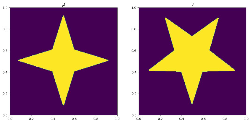
Read from data, black is large pixel

mu = 1-plt.imread('../../images/star.png')[:, :, 2]
nu = 1-plt.imread('../../images/fivestar.png')[:, :, 2]

# Grid of size n1 x n2
output_dim = (256,256)
numIters = 40

mu = process_image(mu,output_dim,sharpen=True)
nu = process_image(nu,output_dim,sharpen=True)

n1, n2 = mu.shape
print('[n1,n2]=',[n1,n2])

x, y = np.meshgrid(np.linspace(0.5 / n1, 1 - 0.5 / n1, n1), np.linspace(0.5 / n2, 1 - 0.5 / n2, n2))
# phi = 0.5 * (x * x + y * y).flatten()
# psi = 0.5 * (x * x + y * y).flatten()
phi = 0.5 * (x * x + y * y)
psi = 0.5 * (x * x + y * y)

#-----------------#
fig, ax = plt.subplots(1, 2)
ax[0].imshow(mu, origin='lower', extent=(0, 1, 0, 1))
ax[0].set_title("$\\mu$")
ax[1].imshow(nu, origin='lower', extent=(0, 1, 0, 1))
ax[1].set_title("$\\nu$")

sigma = 4 / np.maximum(mu.max(), nu.max())

[n1,n2]= [256, 256]

tic = time()
bf = BFM(n1, n2, mu)
compute_ot(phi, psi, bf, sigma)
toc = time()
print(f'\nElapsed time: {toc - tic:.2f}s')

iter    0,   W2 value: 1.336392e-04,   H1 err: 4.73e-04
iter    5,   W2 value: 1.330798e-03,   H1 err: 3.46e-04
iter   10,   W2 value: 2.123883e-03,   H1 err: 1.22e-04
iter   15,   W2 value: 2.636634e-03,   H1 err: 5.47e-05
iter   20,   W2 value: 3.051958e-03,   H1 err: 5.48e-05
iter   25,   W2 value: 3.466675e-03,   H1 err: 5.48e-05
iter   30,   W2 value: 3.881153e-03,   H1 err: 5.48e-05
iter   35,   W2 value: 4.295614e-03,   H1 err: 5.48e-05
iter   40,   W2 value: 4.710060e-03,   H1 err: 5.48e-05

Elapsed time: 13.39s

Lets plot the source and target image.

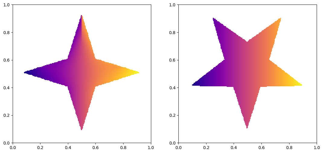
my, mx = ma.masked_array(np.gradient(psi.reshape((n2, n1)) - 0.5 * (x * x + y * y), 1 / n2, 1 / n1), mask=((mu == 0), (mu == 0)))

fig, ax = plt.subplots(1, 2)
ax[0].imshow((x + mx).reshape((n2, n1)), origin='lower', extent=(0, 1, 0, 1), cmap='plasma')
x_masked = ma.masked_array(x, mask=(nu == 0))
ax[1].imshow(x_masked, origin='lower', extent=(0, 1, 0, 1), cmap='plasma')

<matplotlib.image.AxesImage at 0x17cefcbe0>

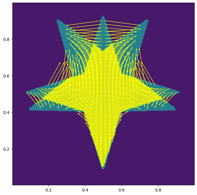
Now we draw the transformation.

fig, ax = plt.subplots()
ax.contourf(x, y, mu + nu)
ax.set_aspect('equal')
skip = (slice(None, None, n1 // 50), slice(None, None, n2 // 50))
ax.quiver(x[skip], y[skip], mx[skip], my[skip], color='yellow', angles='xy', scale_units='xy', scale=1)

<matplotlib.quiver.Quiver at 0x17d08fe20>

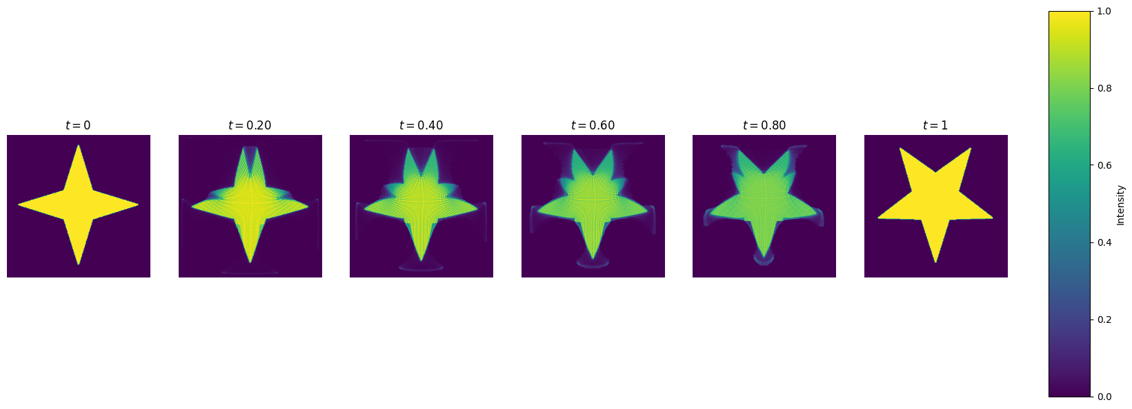
Let’s draw the snapshots of the transformation.

def plot_interpolation(mu, nu, phi, psi, bf, x, y, n_fig=6):
    """
    Plots the discrete geodesic interpolation between mu and nu
    using the given potentials phi and psi.
    
    Parameters
    ----------
    mu : 2D array (n2, n1)
        Source measure.
    nu : 2D array (n2, n1)
        Target measure.
    phi, psi : 2D arrays (n2, n1)
        Kantorovich potentials.
    bf : BFM object
        Instance of the Semi-discrete solver that has a pushforward method.
    x, y : 2D arrays (n2, n1)
        Grid coordinates.
    n_fig : int
        Number of frames to plot (including t=0 and t=1).
    """
    fig, ax = plt.subplots(1, n_fig, figsize=(20, 8))
    for axi in ax:
        axi.axis('off')

    # Use the same max for color scaling
    vmax = max(mu.max(), nu.max())

    # Show the initial and final measures
    im0 = ax[0].imshow(mu, origin='lower', extent=(0, 1, 0, 1), vmax=vmax)
    ax[0].set_title("$t=0$")

    ax[n_fig - 1].imshow(nu, origin='lower', extent=(0, 1, 0, 1), vmax=vmax)
    ax[n_fig - 1].set_title("$t=1$")

    # Allocate arrays for intermediate pushforwards
    interpolate = np.zeros_like(mu)
    rho_fwd = np.zeros_like(mu)
    rho_bwd = np.zeros_like(mu)

    # "Reference" potential = 0.5*(x² + y²)
    phi_0 = 0.5 * (x**2 + y**2)

    # Generate intermediate frames
    for i in range(1, n_fig - 1):
        t = i / (n_fig - 1)

        # Blend potentials in 2D form
        # psi_t interpolates from phi_0 to psi
        # phi_t interpolates from phi_0 to phi
        psi_t = (1 - t) * phi_0 + t * psi
        phi_t = t * phi_0 + (1 - t) * phi

        # Pushforward mu by psi_t
        bf.pushforward(rho_fwd, psi_t, mu)

        # Pushforward nu by phi_t
        bf.pushforward(rho_bwd, phi_t, nu)

        # Convex combination of the two pushforwards
        interpolate = (1 - t) * rho_fwd + t * rho_bwd

        # Plot the interpolation
        ax[i].imshow(interpolate, origin='lower', extent=(0, 1, 0, 1), vmax=vmax)
        ax[i].set_title(f"$t={t:.2f}$")

    # Adjust the main subplot layout to leave room for a dedicated colorbar axis
    plt.subplots_adjust(right=0.85)  # Shrink subplots to make room on the right

    # Create a new axis for the colorbar (position: [left, bottom, width, height])
    cbar_ax = fig.add_axes([0.88, 0.15, 0.03, 0.7])
    fig.colorbar(im0, cax=cbar_ax, label='Intensity')

    plt.show()

plot_interpolation(mu, nu, phi, psi, bf, x, y)
plt.show()